Tensorflow: Natural Language Processing (P1)

This is a brief practice of natural language processing with tensorflow 2.0 high level API. The example is based on “Tensorflow in Practice Specialization” from deeplearning.ai.

In this example, we will use deep neural network to classify a set of sentences to acitve or negative. The dataset is from https://www.kaggle.com/kazanova/sentiment140. We’ll also use transfer learning to help us improve the peformance, which takes place in the embedding layer (vetorize the words in feature space). The embeddings that we will transfer learn from are called the GloVe, also known as Global Vectors for Word Representation, without which we’ll have to train the embeddings ourselves.

00: Import Modules and Set Hyper-parameters

import json
import tensorflow as tf
import csv
import random
import numpy as np

from tensorflow.keras.preprocessing.text import Tokenizer
from tensorflow.keras.preprocessing.sequence import pad_sequences
from tensorflow.keras.utils import to_categorical
from tensorflow.keras import regularizers


embedding_dim = 100 # num of embedding feature dimensions (like RGB for image)
max_length = 16 # max length of a sentence
trunc_type='post' # truncate end words
padding_type='post' # pad in the end
oov_tok = "<OOV>" # out-of-value token
training_size=160000 
test_portion=.1 # 10% data for test

corpus = []

01: Prepare Data

We first download data and extract sentences and labels

!wget --no-check-certificate \
    https://storage.googleapis.com/laurencemoroney-blog.appspot.com/training_cleaned.csv \
    -O /tmp/training_cleaned.csv

--2020-08-20 15:12:32--  https://storage.googleapis.com/laurencemoroney-blog.appspot.com/training_cleaned.csv
Resolving storage.googleapis.com (storage.googleapis.com)... 173.194.69.128, 173.194.79.128, 108.177.119.128, ...
Connecting to storage.googleapis.com (storage.googleapis.com)|173.194.69.128|:443... connected.
HTTP request sent, awaiting response... 200 OK
Length: 238942690 (228M) [application/octet-stream]
Saving to: ‘/tmp/training_cleaned.csv’

/tmp/training_clean 100%[===================>] 227.87M  70.3MB/s    in 3.2s    

2020-08-20 15:12:36 (70.3 MB/s) - ‘/tmp/training_cleaned.csv’ saved [238942690/238942690]

num_sentences = 0

with open("/tmp/training_cleaned.csv") as csvfile:
    reader = csv.reader(csvfile, delimiter=',')
    for row in reader:
        list_item=[]
        list_item.append(row[5])
        this_label=row[0]
        if this_label=='0': # binary class
            list_item.append(0)
        else:
            list_item.append(1)
        num_sentences = num_sentences + 1
        corpus.append(list_item)

Have a look at the sentences.

print(num_sentences)
print(len(corpus))
print(corpus[0])

1600000
1600000
['@MilkyMooMoo Oh no, my old mum wont let me use the phone on mondays and certainly not to ring a pretty lady like you! ', 1]

Prepare training data.

# create sentences and labels
sentences=[]
labels=[]
random.shuffle(corpus)
for x in range(training_size):
    sentences.append(corpus[x][0])
    labels.append(corpus[x][1])

# tokenize the sentences: word --> index
tokenizer = Tokenizer()
tokenizer.fit_on_texts(sentences)

word_index = tokenizer.word_index
vocab_size=len(word_index) # num of different words

sequences = tokenizer.texts_to_sequences(sentences) # transfer a sentence to an index sequence
padded = pad_sequences(sequences, maxlen=max_length, padding=padding_type, truncating=trunc_type) # form all sentence sequences to the same length

# split the sequences to training and test
split = int(test_portion * training_size) 

test_sequences = padded[0:split]
training_sequences = padded[split:training_size]
test_labels = labels[0:split]
training_labels = labels[split:training_size]

02: Build model from transfer learning

We first download and generate Glove embedding model.

# Note this is the 100 dimension version of GloVe from Stanford
# I unzipped and hosted it on my site to make this notebook easier
!wget --no-check-certificate \
    https://storage.googleapis.com/laurencemoroney-blog.appspot.com/glove.6B.100d.txt \
    -O /tmp/glove.6B.100d.txt

--2020-08-20 15:13:02--  https://storage.googleapis.com/laurencemoroney-blog.appspot.com/glove.6B.100d.txt
Resolving storage.googleapis.com (storage.googleapis.com)... 108.177.119.128, 108.177.126.128, 108.177.127.128, ...
Connecting to storage.googleapis.com (storage.googleapis.com)|108.177.119.128|:443... connected.
HTTP request sent, awaiting response... 200 OK
Length: 347116733 (331M) [text/plain]
Saving to: ‘/tmp/glove.6B.100d.txt’

/tmp/glove.6B.100d. 100%[===================>] 331.04M  62.4MB/s    in 5.3s    

2020-08-20 15:13:08 (62.4 MB/s) - ‘/tmp/glove.6B.100d.txt’ saved [347116733/347116733]

embeddings_index = {}
with open('/tmp/glove.6B.100d.txt',encoding='utf-8') as f:
    for line in f:
        values = line.split()
        word = values[0]
        coefs = np.asarray(values[1:], dtype='float32')
        embeddings_index[word] = coefs

embeddings_matrix = np.zeros((vocab_size+1, embedding_dim)); # storing the word embedding info
for word, i in word_index.items():
    embedding_vector = embeddings_index.get(word)
    if embedding_vector is not None:
        embeddings_matrix[i] = embedding_vector

Then build the network model with both convolution and LSTM layers.

model = tf.keras.Sequential([
    tf.keras.layers.Embedding(vocab_size+1, embedding_dim, input_length=max_length, weights=[embeddings_matrix], trainable=False), # set parameters of pre-loaded embedding model untrainable
    tf.keras.layers.Dropout(0.2),
    tf.keras.layers.Conv1D(64, 5, activation='relu'),
    tf.keras.layers.MaxPooling1D(pool_size=4),
    tf.keras.layers.LSTM(64),
    tf.keras.layers.Dense(1, activation='sigmoid')
])
model.compile(loss='binary_crossentropy',optimizer='adam',metrics=['accuracy'])
model.summary()

Model: "sequential"
_________________________________________________________________
Layer (type)                 Output Shape              Param #   
=================================================================
embedding (Embedding)        (None, 16, 100)           13912200  
_________________________________________________________________
dropout (Dropout)            (None, 16, 100)           0         
_________________________________________________________________
conv1d (Conv1D)              (None, 12, 64)            32064     
_________________________________________________________________
max_pooling1d (MaxPooling1D) (None, 3, 64)             0         
_________________________________________________________________
lstm (LSTM)                  (None, 64)                33024     
_________________________________________________________________
dense (Dense)                (None, 1)                 65        
=================================================================
Total params: 13,977,353
Trainable params: 65,153
Non-trainable params: 13,912,200
_________________________________________________________________

03: Training and Visualization

Before training, we have to transfer the senquences and labels into numpy arrays.

num_epochs = 50

training_padded = np.array(training_sequences)
training_labels = np.array(training_labels)
testing_padded = np.array(test_sequences)
testing_labels = np.array(test_labels)

history = model.fit(training_padded, training_labels, epochs=num_epochs, validation_data=(testing_padded, testing_labels), verbose=2)

print("Training Complete")

Epoch 1/50
4500/4500 - 16s - loss: 0.5665 - accuracy: 0.6995 - val_loss: 0.5379 - val_accuracy: 0.7274
Epoch 2/50
4500/4500 - 15s - loss: 0.5254 - accuracy: 0.7333 - val_loss: 0.5205 - val_accuracy: 0.7404
Epoch 3/50
4500/4500 - 15s - loss: 0.5092 - accuracy: 0.7442 - val_loss: 0.5226 - val_accuracy: 0.7416
Epoch 4/50
4500/4500 - 15s - loss: 0.4984 - accuracy: 0.7527 - val_loss: 0.5139 - val_accuracy: 0.7457
Epoch 5/50
4500/4500 - 15s - loss: 0.4890 - accuracy: 0.7584 - val_loss: 0.5118 - val_accuracy: 0.7493
......
Epoch 46/50
4500/4500 - 15s - loss: 0.4248 - accuracy: 0.7987 - val_loss: 0.5381 - val_accuracy: 0.7418
Epoch 47/50
4500/4500 - 15s - loss: 0.4236 - accuracy: 0.7988 - val_loss: 0.5361 - val_accuracy: 0.7429
Epoch 48/50
4500/4500 - 15s - loss: 0.4265 - accuracy: 0.7964 - val_loss: 0.5338 - val_accuracy: 0.7426
Epoch 49/50
4500/4500 - 15s - loss: 0.4246 - accuracy: 0.7984 - val_loss: 0.5375 - val_accuracy: 0.7434
Epoch 50/50
4500/4500 - 15s - loss: 0.4244 - accuracy: 0.7978 - val_loss: 0.5393 - val_accuracy: 0.7437
Training Complete

Let’s have a look at the training process, watching how accuracy and loss change over epochs.

import matplotlib.image  as mpimg
import matplotlib.pyplot as plt

#-----------------------------------------------------------
# Retrieve a list of list results on training and test data
# sets for each training epoch
#-----------------------------------------------------------
acc=history.history['accuracy']
val_acc=history.history['val_accuracy']
loss=history.history['loss']
val_loss=history.history['val_loss']

epochs=range(len(acc)) # Get number of epochs

#------------------------------------------------
# Plot training and validation accuracy per epoch
#------------------------------------------------
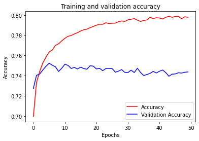
plt.plot(epochs, acc, 'r')
plt.plot(epochs, val_acc, 'b')
plt.title('Training and validation accuracy')
plt.xlabel("Epochs")
plt.ylabel("Accuracy")
plt.legend(["Accuracy", "Validation Accuracy"])

plt.figure()

#------------------------------------------------
# Plot training and validation loss per epoch
#------------------------------------------------
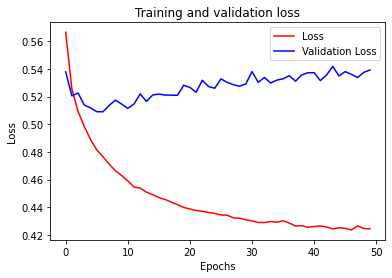
plt.plot(epochs, loss, 'r')
plt.plot(epochs, val_loss, 'b')
plt.title('Training and validation loss')
plt.xlabel("Epochs")
plt.ylabel("Loss")
plt.legend(["Loss", "Validation Loss"])

plt.figure()


# Expected Output
# A chart where the validation loss does not increase sharply!

<Figure size 432x288 with 0 Axes>

<Figure size 432x288 with 0 Axes>

We can see that the training accuracy reaches up to 80%, which is quite good. However, there exists some kind of overfitting.

04: Use the model

Let’s try this trained model to classify some sentences.

test_0 = ["I love you","I hate you","You're a good man, but we are not suitable to be together."]
test_1 = tokenizer.texts_to_sequences(test_0)
test_2 = pad_sequences(test_1, maxlen=max_length, padding=padding_type, truncating=trunc_type)
test_3 = np.array(test_2)
re = model.predict(test_3)
for i in range(len(re)):
  print(re[i])
  if re[i]>0.8:
    print('positive')
  elif re[i]<0.2:
    print('negative')

[0.88264596]
positive
[0.03774856]
negative
[0.24521422]

Both are classified correctly, the third is also reasonable. It’s not bad:)