Tensorflow: Time Sequences (P1)

This is a brief practice of time sequence processing with tensorflow 2.0 high level API. The example is based on “Tensorflow in Practice Specialization” from deeplearning.ai.

In this example, we will practice generating simulated time sequence data and doing a regression using recurrent neural network. In the next blog, we’ll try to deal with real-world data.

00: Set up

import tensorflow as tf
import numpy as np
import matplotlib.pyplot as plt
print(tf.__version__)

2.3.0

01: Prepare Data

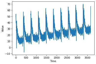
A common time series contains the base value, a self-directed trend or autocorrelation, a seasonal pattern and some noise. In this part, we create a simulated time series.

def plot_series(time, series, format="-", start=0, end=None):
    plt.plot(time[start:end], series[start:end], format)
    plt.xlabel("Time")
    plt.ylabel("Value")
    plt.grid(False)

def trend(time, slope=0):
    return slope * time

def seasonal_pattern(season_time):
    """Just an arbitrary pattern, you can change it if you wish"""
    return np.where(season_time < 0.1,
                    np.cos(season_time * 6 * np.pi),
                    2 / np.exp(9 * season_time))

def seasonality(time, period, amplitude=1, phase=0):
    """Repeats the same pattern at each period"""
    season_time = ((time + phase) % period) / period
    return amplitude * seasonal_pattern(season_time)

def noise(time, noise_level=1, seed=None):
    rnd = np.random.RandomState(seed)
    return rnd.randn(len(time)) * noise_level

time = np.arange(10 * 365 + 1, dtype="float32")
baseline = 10
series = trend(time, 0.1)  
baseline = 10
amplitude = 40
slope = 0.005
noise_level = 3

# Create the series
series = baseline + trend(time, slope) + seasonality(time, period=365, amplitude=amplitude)
# Update with noise
series += noise(time, noise_level, seed=51)

split_time = 3000
time_train = time[:split_time]
x_train = series[:split_time]
time_valid = time[split_time:]
x_valid = series[split_time:]

window_size = 20
batch_size = 32
shuffle_buffer_size = 1000

plot_series(time, series)

Then we prepare the training data based on the simulated sequence. Each training-label pair contains a batch of windowed time sequence and the next time-stamp value.

def windowed_dataset(series, window_size, batch_size, shuffle_buffer):
  dataset = tf.data.Dataset.from_tensor_slices(series)
  dataset = dataset.window(window_size + 1, shift=1, drop_remainder=True)
  dataset = dataset.flat_map(lambda window: window.batch(window_size + 1))
  dataset = dataset.shuffle(shuffle_buffer).map(lambda window: (window[:-1], window[-1]))
  dataset = dataset.batch(batch_size).prefetch(1)
  return dataset

tf.keras.backend.clear_session()
tf.random.set_seed(51)
np.random.seed(51)
dataset = windowed_dataset(x_train, window_size, batch_size, shuffle_buffer_size)

02: Build Model

We build a sequential model with LSTM layers. The Lambda layer enables the layer being customized, here used for changing the input data shape.

tf.keras.backend.clear_session()

model = tf.keras.models.Sequential([
  tf.keras.layers.Lambda(lambda x: tf.expand_dims(x, axis=-1), input_shape=[None]),
  tf.keras.layers.Bidirectional(tf.keras.layers.LSTM(32, return_sequences=True)),
  tf.keras.layers.Bidirectional(tf.keras.layers.LSTM(32)),
  tf.keras.layers.Dense(1),
  tf.keras.layers.Lambda(lambda x: x * 100.0)
])
model.summary()

Here we introcude a simple method to choose a suitable learning rate. We set different learning rates and do the training, then plot the losses w.r.t learning rates, and choose the smallest one.

lr_schedule = tf.keras.callbacks.LearningRateScheduler(
    lambda epoch: 1e-8 * 10**(epoch / 20))
optimizer = tf.keras.optimizers.SGD(lr=1e-8, momentum=0.9)
model.compile(loss=tf.keras.losses.Huber(),
              optimizer=optimizer,
              metrics=["mae"])
history = model.fit(dataset, epochs=100, callbacks=[lr_schedule])

Epoch 1/100
94/94 [==============================] - 1s 12ms/step - loss: 8.5331 - mae: 9.0204
Epoch 2/100
94/94 [==============================] - 1s 11ms/step - loss: 8.0548 - mae: 8.5392
Epoch 3/100
94/94 [==============================] - 1s 11ms/step - loss: 7.7249 - mae: 8.2080
Epoch 4/100
94/94 [==============================] - 1s 11ms/step - loss: 7.5026 - mae: 7.9862
Epoch 5/100
94/94 [==============================] - 1s 11ms/step - loss: 7.3488 - mae: 7.8287
......
Epoch 96/100
94/94 [==============================] - 1s 10ms/step - loss: 3.6194 - mae: 4.0909
Epoch 97/100
94/94 [==============================] - 1s 10ms/step - loss: 3.9668 - mae: 4.4424
Epoch 98/100
94/94 [==============================] - 1s 10ms/step - loss: 4.0499 - mae: 4.5214
Epoch 99/100
94/94 [==============================] - 1s 10ms/step - loss: 5.6996 - mae: 6.1759
Epoch 100/100
94/94 [==============================] - 1s 10ms/step - loss: 5.3132 - mae: 5.7924

plt.semilogx(history.history["lr"], history.history["loss"])
plt.axis([1e-8, 1e-4, 0, 30])

# FROM THIS PICK A LEARNING RATE

(1e-08, 0.0001, 0.0, 30.0)

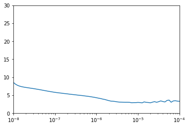
From the figure above we can see 1e-5 performs well, so we set it as our learning rate.

03: Training and Visualization

Now we rebuild the same model and use the chosen learning rate to do the training.

tf.keras.backend.clear_session()

model = tf.keras.models.Sequential([
  tf.keras.layers.Lambda(lambda x: tf.expand_dims(x, axis=-1), input_shape=[None]),
  tf.keras.layers.Bidirectional(tf.keras.layers.LSTM(32, return_sequences=True)),
  tf.keras.layers.Bidirectional(tf.keras.layers.LSTM(32)),
  tf.keras.layers.Dense(1),
  tf.keras.layers.Lambda(lambda x: x * 100.0)
])

model.compile(loss="mse", optimizer=tf.keras.optimizers.SGD(lr=1e-5, momentum=0.9),metrics=["mae"])
history = model.fit(dataset,epochs=500,verbose=1)
                                                      

Epoch 1/500
94/94 [==============================] - 1s 10ms/step - loss: 263.1988 - mae: 10.1378
Epoch 2/500
94/94 [==============================] - 1s 10ms/step - loss: 33.6153 - mae: 3.9017
Epoch 3/500
94/94 [==============================] - 1s 11ms/step - loss: 27.7103 - mae: 3.5518
Epoch 4/500
94/94 [==============================] - 1s 10ms/step - loss: 31.9160 - mae: 3.9759
Epoch 5/500
94/94 [==============================] - 1s 10ms/step - loss: 27.1127 - mae: 3.5515
......
Epoch 496/500
94/94 [==============================] - 1s 10ms/step - loss: 19.6845 - mae: 2.9502
Epoch 497/500
94/94 [==============================] - 1s 10ms/step - loss: 19.3691 - mae: 2.9267
Epoch 498/500
94/94 [==============================] - 1s 10ms/step - loss: 19.7436 - mae: 2.9396
Epoch 499/500
94/94 [==============================] - 1s 10ms/step - loss: 20.6016 - mae: 3.0397
Epoch 500/500
94/94 [==============================] - 1s 10ms/step - loss: 19.3550 - mae: 2.9032

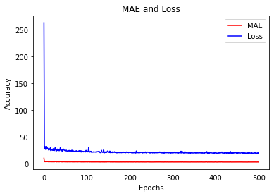
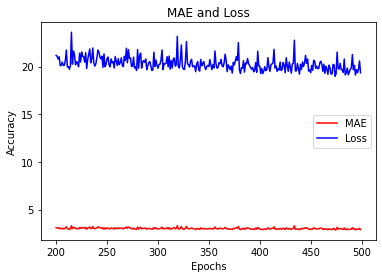
Let’s have a look at the training losses over epochs.

import matplotlib.image  as mpimg
import matplotlib.pyplot as plt

#-----------------------------------------------------------
# Retrieve a list of list results on training and test data
# sets for each training epoch
#-----------------------------------------------------------
mae=history.history['mae']
loss=history.history['loss']

epochs=range(len(loss)) # Get number of epochs

#------------------------------------------------
# Plot MAE and Loss
#------------------------------------------------
plt.plot(epochs, mae, 'r')
plt.plot(epochs, loss, 'b')
plt.title('MAE and Loss')
plt.xlabel("Epochs")
plt.ylabel("Accuracy")
plt.legend(["MAE", "Loss"])

plt.figure()

epochs_zoom = epochs[200:]
mae_zoom = mae[200:]
loss_zoom = loss[200:]

#------------------------------------------------
# Plot Zoomed MAE and Loss
#------------------------------------------------
plt.plot(epochs_zoom, mae_zoom, 'r')
plt.plot(epochs_zoom, loss_zoom, 'b')
plt.title('MAE and Loss')
plt.xlabel("Epochs")
plt.ylabel("Accuracy")
plt.legend(["MAE", "Loss"])

plt.figure()

<Figure size 432x288 with 0 Axes>

<Figure size 432x288 with 0 Axes>

04: Use the model

Let’s use the model to predict regressed values and compare that to our validation data.

forecast = []
results = []
for time in range(len(series) - window_size):
  forecast.append(model.predict(series[time:time + window_size][np.newaxis]))

forecast = forecast[split_time-window_size:]
results = np.array(forecast)[:, 0, 0]


plt.figure(figsize=(10, 6))

plot_series(time_valid, x_valid)
plot_series(time_valid, results)

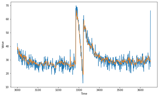
tf.keras.metrics.mean_absolute_error(x_valid, results).numpy()

2.920534

The result looks quite good with a mean absolute error of 2.92. In the next blog, we will have a practice on real-world data.